INTRODUCTION & GENERAL NOTES
Balmoral Software
INTRODUCTION & GENERAL NOTES
Balmoral Software
Notation
The following notation is used on these pages:
S: Closed curve in the plane (may be convex or non-convex)In spite of its idiosyncrasies and the frequent need to "tease" answers from it, WolframAlpha is widely used for numerical integration and some of the mathematical heavy lifting in order to condense the various analyses presented on these pages. Future efforts may leverage SymPy.
R: Radius of a boundary circle
A: Area enclosed by a closed curve
L: Arc length (perimeter) of a closed curve
a: Semiwidth of a boundary ellipse
b: Semiheight of a boundary ellipse (a and b are referred to as the dimensions of the ellipse)
(c,d): Coordinates of the center of a boundary conic
t: A parameter by which S is defined, analogous to time or angle
T: The domain interval for t, typically [0,2π)
tR: Rotation angle
x(t), y(t): Parametric functions defining the cartesian coordinates of a curve's path
r(t): Polar radius function defining the radial distance of S from the origin as a function of radial angle t
φ: Alternate representation of radial angle
β: Apex angle of a triangle
F(x,y): Implicit function describing a closed curve
(xc,yc): Coordinates of the centroid of S
w: Width of an isosceles triangle
h: Height of an isosceles triangle
m: Slope of a line
z: Axis intercept
x(t) = 2cos(t) + cos(2t)for t ∈ T = [0,2π). In general, the parameter t does not correspond to the angle that the point (x(t),y(t)) makes with respect to the origin and the positive x-axis, and it may be convenient to consider x(t) and y(t) as functions of elapsed time t as a point traverses the curve.y(t) = 2sin(t) - sin(2t)
Alternatively, S can be defined in terms of a polar radius function r(t), which describes the radial distance from a point on S to the origin at an angle t measured counterclockwise from the positive x-axis. For example, the bifolium described by the black curve in the diagram above is defined by its polar radius function
r(t) = sin(t)cos2(t), 0 ≤ t < πThe corresponding cartesian coordinate functions are defined by
x(t) = r(t)cos(t)for t ∈ T. The reverse operation of converting parametric coordinate functions into a polar coordinate function is generally not possible unless the ratio of x(t) and y(t) is a tangent.y(t) = r(t)sin(t)
A curve S may also be expressed implicitly in terms of a function
F(x,y) = (x2 + y2)2 - 4x2 - y2 = 0If F is separable and can be expressed in the form
x(t) = tA closed curve frequently has more than one of polar, parametric and implicit representations, which can be used to determine its symmetry.y(t) = G[x(t)]
Scaling
Definitions of closed curves on these pages are usually chosen in their simplest or standard form without scaling parameter(s); exceptions are a few specific curves that will be compared with others that are similar in shape.
Metric formulas
All equation numbers on the individual curve pages on this site refer to this Introduction, the formulas for which are defined in sections below:
(L1),(L2): Arc length formulas for polar and parametric curves
(A1),(A2): Area formulas for polar and parametric curves
(C1),(C2): Centroid formulas for polar and parametric curves
(R1),(R2): Rotational symmetry conditions for polar and parametric curves
(X1),(X2): Curvature and tangent slope formulas
(r,-t) also satisfies the polar formulaAn example is the cardioid. Analogously, S is symmetric with respect to the y-axis (y-symmetric) when
(-r,-t) also satisfies the polar formulaAn example is the bifolium. If S is symmetric with respect to both coordinate axes, it is said to be bisymmetric; an example is the nephroid. Note that if the exponent of r is odd in the polar formula, then S cannot be bisymmetric. The table below presents symmetries of closed curves defined by a polar formula:
Polar curves
If a closed curve S is defined by an implicit cartesian function of the formNote 1: r = sin3(t + π/4) + cos3(t + π/4) is an even function
S Polar formula x-symmetric y-symmetric Tschirnhausen cubic r = sec3(t/3) ✓ Right strophoid r = cos(2t)sec(t) ✓ Trisectrix of Maclaurin r = 4cos(t) - sec(t) ✓ Bifolium r = sin(t)cos2(t) ✓ Hippopede r2 = 4 - 3sin2(t) ✓ ✓ Dipole r2 = cos(t) ✓ ✓ Lemniscate of Gerono r2 = cos(2t)sec4(t) ✓ ✓ Trefoil r = cos(t)cos(2t) ✓ Lima bean curve (rotated) (Note 1) ✓ Cardioid r = 1 - cos(t) ✓ Cochleoid r = -2sin(t)/t ✓ Cayley sextic r = -2cos3(t/3) ✓ Rose r = cos(3t) ✓ Deltoid r4 + 18r2 - 27 = 8r3cos(3t) ✓
Implicit curves
Applying the rules of symmetry for polar functions to parametric functions, S is x-symmetric when:*: See bowtie page
S Implicit function F(x,y) x-symmetric y-symmetric Piriform curve y2 - 2x3 - x4 ✓ Bicorn y2(1 - x2) - (x2 + 2y - 1)2 ✓ Bernoulli (x2 + y2)2 - 2(x2 - y2) ✓ ✓ Bowtie (rotated) (x2 + y2)3 - (3x2 - y2)2 * ✓ ✓ Dumbbell curve y2 - x4 + x6 ✓ ✓ Fish curve ✓ Nephroid (x2 + y2 - 4)3 - 108y2 ✓ ✓ Mouth y2 - (1 - x2)3 ✓ ✓
(r,-t) satisfies the polar formulaS is y-symmetric when:
x(-t) = rcos(-t) = rcos(t) = x(t) (x is an even function)
y(-t) = rsin(-t) = -rsin(t) = -y(t) (y is an odd function)
(-r,-t) satisfies the polar formulaParametric curves
x(-t) = -rcos(-t) = -rcos(t) = -x(t) (x is an odd function)
y(-t) = -rsin(-t) = r(t)sin(t) = y(t) (y is an even function)
Several closed curves with piecewise definitions have symmetries by construction:
S x(t) y(t) x-symmetric y-symmetric Teardrop curve -cos(t) sin(t)sin2(t/2) ✓ Epicycloid 4cos(t)-cos(4t) 4sin(t) - sin(4t) ✓ Heart curve 16sin3(t) 13cos(t) - 5cos(2t) - 2cos(3t) -cos(4t) ✓
Piecewise-defined curves
Finally, S is rotationally symmetric if r is a periodic function for some offset α:
S x-symmetric y-symmetric Arbelos Lune ✓ Cycloid arches ✓ ✓ Vesica Piscis ✓ ✓ Isosceles triangle ✓ Circular sector ✓ Circular segment ✓
r(t + α) = r(t)If S is rotationally symmetric with a period of less than π (that is, containing three or more lobes, cusps or corners), its circumellipse and circumcircle are the same. An example is the deltoid.
Clearly, if S is bisymmetric or rotationally symmetric and is not self-intersecting, its incircle and circumcircle are concentric.
By the symmetry principle [2], boundary conics have the same symmetry as S since what is optimal in one half-plane will be optimal in the other. Therefore, their centers will lie on the axis of symmetry. Similar remarks apply to the convex hull of S.
Self-intersection
Any closed curve that is self-intersecting (not simple) is non-convex. Such a curve passes through the same point more than once over its parameter domain. Examples include the fish curve and a rose with any number of petals.
Multiple local coordinate extrema
A simple curve S is not convex if there is more than one local minimum or maximum abscissa or ordinate. In the example below, two maximum ordinates exist:
In these cases, the convex hull of S is constructed by adding horizontal or vertical line segments between the local coordinate extrema, as shown in blue above. Examples are the cardioid and the bifolium. Rotationally-symmetric non-convex shapes such as an epicycloid with 3 or more lobes may have additional convex hull line segments added.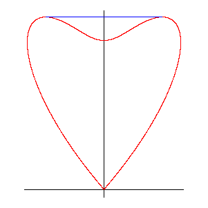
A simple closed curve S is not convex in the neighborhood of a point where its curvature changes sign. Such curves typically have a symmetry that forms a cusp (u,v) at one or more points of zero curvature. One example is the piriform curve, which has zero curvature above, below and at the cusp at the origin. Another example is the heart curve, which has zero curvature at its lower cusp and at two symmetric points above it. If S is defined by parametric coordinate functions x(t) and y(t), its signed curvature is zero when
In these cases, the convex hull is constructed by adding one or more line segments, each of which encloses a zero-curvature point, has one endpoint at the cusp and is tangent to S at its other endpoint. The point P at which the curvature of S changes sign is interior to the convex hull, as seen in the diagram below:
x'(t)y''(t) = x''(t)y'(t) for some t ∈ T (X1)
The slope of the tangent line equals the ratio of offsets between the points of tangency: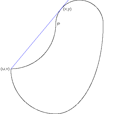
Equation (X2) is solved for t in order to define the endpoint (x(t),y(t)) of the convex hull line segment. Note that this endpoint often coincides with the point of tangency of S and its inellipse, such as in the piriform, teardrop and mouth curves, but an exception is the heart curve.
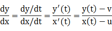
(X2)
Most of the curves considered on these pages are non-convex.
Some definitions of an optimal circumconic or inconic characterize it as having the minimum or maximum perimeter, respectively, of all bounding or bounded conics. However, this can lead to impracticalities for certain shapes, as will be shown next. Instead, optimal boundary ellipses on these pages are determined by their area. In the case of boundary circles, optimizing perimeter and area are equivalent since both are defined by a single radius variable.
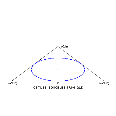
For example, the maximum perimeter of an ellipse inscribed in an obtuse
isosceles triangle is achieved when the ellipse is a degenerate one coincident
with the base of the triangle. Conversely, the maximum area of the
inscribed ellipse occurs when the ellipse is tangent to the triangle at an
intermediate point on each side. To see this, let the triangle have base width
w and height h,
b = h(1/2 - 2a2/w2)The area of the inellipse
A = abπ = h(a/2 - 2a3/w2)πis maximized when
as shown in blue on the left diagram below.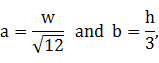
Conversely, the perimeter of the inscribed ellipse has a lower bound [3]
π(a + b) = π[a + h(1/2 - 2a2/w2)],which is maximized when
a = w/2 and b = 0,which in turn results in a degenerate ellipse with perimeter 2w at the triangle base, shown in red in the left diagram below:
Because of this unrepresentative effect that can occur in such shapes as the bicorn and the circular segment, optimization of inconics on these pages is based on maximizing area rather than perimeter. For consistency, optimization of circumconics is based analogously on minimizing area. This approach produces better-fitting boundary conics over a variety of shapes, as well as providing closed-form results in many cases.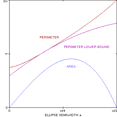
Boundary Conics
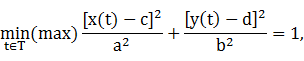
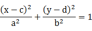
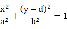
The inequality
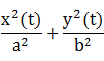
describes all points (x,y) that are on or inside an axis-aligned ellipse with semiwidth a, semiheight b and center (c,d). If the left side of (1) is
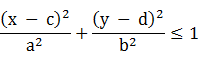
(1)
then the aforementioned ellipse is an inellipse (circumellipse) of the curve described by the parametric functions x(t) and y(t). Similarly, a circle with radius R and center (c,d) for which
(2)
is an incircle (circumcircle) of S. Boundary conics are found by optimizing the area of all candidates that satisfy (2) or (3). Clearly, the center point (c,d) of a boundary conic occurs within the bounding rectangle of S.
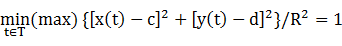
(3)
Algorithms
In practice, closed-form results for optimal boundary conics are found using some fundamental algorithms described in the Appendix. The application of these algorithms varies according to the symmetry of S. In some cases, the best-fitting boundary conic is found by using its tangency at a cusp or extreme edge of S, as described in Lemmas C and E, then verifying using a method in the preceding section and confirming with a numerical search as described below.
In the case of a bisymmetric curve, the extrema of the squared-radius function
r2(t) or
The squared-radius function is also used to determine the circumcircle (and incircle if it exists) of a rotationally-symmetric curve with a period of less than π. In this case, the circumconics are the same.
If S is x- or y-symmetric, the diameter of its circumcircle may be determined from its ordinate or abscissa extrema, respectively, subject to verification. Limits on the interior space of S along the axis of symmetry may determine its incircle, or it may be determined from a maximum-coordinate point if space on the axis of symmetry permits, in each case subject to the verification step being satisfied. Otherwise, Lemma C can be applied.
The circumellipse and inellipse of an x- or y-symmetric curve are generally found using Lemma E. In a few cases, Lemma E may fail to provide a closed-form solution satisfying the verification step, and a numerical search algorithm such as that described in the next section can be used.
In the first iteration, these parameter ranges are broken into increments of 0.01, with the increment and ranges divided in half for each subsequent iteration. The center of each range is defined as the best value of the corresponding parameter found so far, based on optimizing area and subject to the overall constraints of S. Fifteen iterations are sufficient to converge to an optimal parameter value accurate to 6 decimal places (an error of less than one part in a million). Double precision arithmetic is used throughout.
The algorithm is efficient enough that an additional parameter loop for optimizing the tilt of an arbitrary ellipse can be implemented in a reasonable runtime, offering a numeric solution for the inellipse of an asymmetric arbelos, for example.
The area [5] enclosed by S is
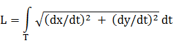
(L1)
Areas of subregions of T are delimited by vertical line segments extending to the x-axis, as in the calculations of the convex hull area of the heart curve.
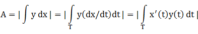
(A1)
If S is described in terms of a polar radius function r(t), then the arc length and area [6] are:
Areas of subregions of T are delimited by radial line segments from the origin, as in the calculations of the convex hull area of the trefoil.
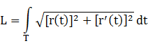
(L2) 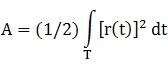
(A2)
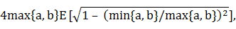
The perimeter of an ellipse with dimensions a and b is
where E is the complete elliptic integral of the second kind, for which a closed-form expression doesn't exist. To provide an accurate approximation of E in (4), the QBASIC algorithm in [7] can be used with double precision arithmetic. For spot checks of ellipse perimeters, the WolframAlpha expression "perimeter of ellipse with a=value and b=value" can be used. We have the following familiar formulas for boundary conics:
(4)
Boundary conic Perimeter Area Circle 2πR πR2 Ellipse Equation (4) πab
where A is the area of S defined by (A1).
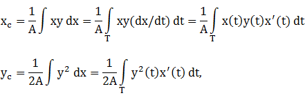
(C1)
For S defined by a polar radius function r(t), the centroid coordinates [9] are:
where A is defined in (A2).
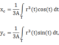
(C2)
Obviously, the centroid of a boundary conic is its center point (c,d).
By the symmetry principle [2], if S is symmetric with respect to a coordinate axis, its centroid and those of its boundary conics lie on that axis. It follows that the common centroid of S and its boundary conics is at the origin when S is bisymmetric.
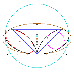
Each closed curve S and its boundary conics and convex hull are plotted on a square polar chart. The following color scheme is used:
Centroids are indicated by an "X" in the corresponding color. Scaling is uniform for both coordinates, and the axis interval is shown.
S & coordinate axes Black Convex hull line segments (if any) Blue Inconic bounding rectangle (if any) Light green Circumcircle Cyan Circumellipse Brown Inellipse Red Incircle Purple Annotations (if any) Green
Radial
S and its associated boundary conics and convex hull are also plotted with the same color scheme on a rectilinear diagram depicting the radial distance from the origin as a function of radial angle φ, measured counterclockwise from the positive x-axis. The corresponding coordinate functions for an ellipse with dimensions a and b centered at (c,d) are
x(φ) = acos(φ) + cCartesian coordinates are converted to angle and radial distance in the usual way:
y(φ) = bsin(φ) + d
where Atan2 is the two-argument arctangent. The domain of φ is 2π wide, chosen to center the diagram.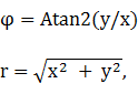
Lemma Description Lemma B Bisymmetric boundary ellipses Lemma C x/y-symmetric boundary circles Lemma E x/y-symmetric boundary ellipses Lemma R Condition for rotational symmetry Lemma S Condition for inellipse = incircle Lemma T Ellipse tangent to a line Lemma TC Circumcircle of y-symmetric isosceles triangle Lemma TE Circumellipse of isosceles triangle Lemma X WolframAlpha arctangent simplification Lemma X2 WolframAlpha arctangent simplification Lemma H Circumconic contains convex hull
is 2, attained at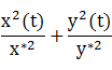
Proof. Since
we have
and the extreme value is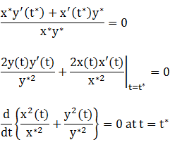
Setting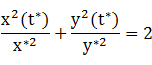
over
has an extremum at 1
but in practice, the outcome is usually obvious by graphing.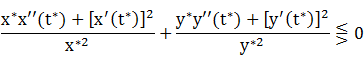
The verification step (2) is subsequently applied.
where the optimization (minimizing or maximizing) is determined by the following table: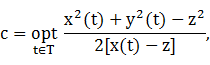
In either case, the radius of the boundary circle is R = |c - z|.
x-symmetric Boundary circle Tangent point Incircle Circumcircle Left edge Minimize Maximize Right edge Maximize Minimize
Analogously, if S is y-symmetric and the tangent point on the y-axis is (0,z), then the center ordinate of the boundary circle is
where the optimization (minimizing or maximizing) is determined by the following table:
In either case, the radius of the boundary circle is R = |d - z|.
y-symmetric Boundary circle Tangent point Incircle Circumcircle Bottom edge Minimize Maximize Top edge Maximize Minimize
The range for optimization can be limited to a subset of T containing the expected points of tangency of the circle and S, which are usually obvious from a polar diagram of S.
Proof: If S is x-symmetric, its circumcircle is the smallest one satisfying the inequality
[x(t) - c]2 + y2(t) ≤ R2 for all t ∈ TSince (z,0) is on S, we have
(z - c)2 ≤ R2so R is minimized at |c - z|. A general point (x(t),y(t)) on S then satisfies
[x(t) - c]2 + y2(t) ≤ (c - z)2,which reduces to
2[x(t) - z]c ≥ x2(t) + y2(t) - z2If z is at the left edge of the curve, then x(t) > z almost everywhere and the preceding inequality becomes
The inequality is satisfied over T if
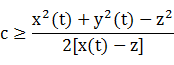
(5)
In the case of an incircle tangent to the left edge of S, the inequalities are reversed and c is minimized over T. Similarly, if the tangent point is at the right edge, the division in (5) is by a negative number and the corresponding inequality is reversed. Hence, we have the x-symmetric table above.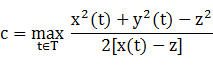
To prove the comparable case for y-symmetric curves, exchange abscissa and ordinate, x and y, c and d in the results above.
an extreme value of
(6)
over T is 1, attained at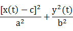
Analogously, if S is y-symmetric with y-intercept (0,z) and
is a candidate for either the inellipse or circumellipse of S.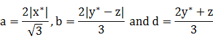
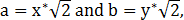
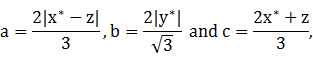
Proof. Assume S is x-symmetric but not bisymmetric (in which case, see Lemma B). Clearly, a boundary ellipse of S has at least three points of tangency with S since fewer would indicate that a more optimal ellipse could be found. By symmetry, two of these tangencies are symmetric with respect to the x-axis. The formulas for a, b and c are derived from Lemma TE through lateral translation by x*. From (6), we have
Since
c - z = 2(x* - z)/3 and x* - c = (x* - z)/3 (7)
the specified ellipse passes through the x-intercept (z,0). We have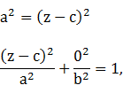
so we can divide by (2/3)(x* - z)y* to get
using (6) and (7). It follows that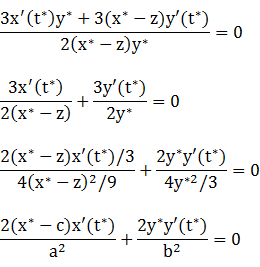
and the extreme value is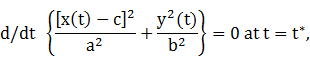
To prove the comparable case for y-symmetric curves, exchange abscissa and ordinates, x and y, a and b, c and d in the results above.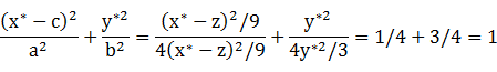
If S is defined by a polar radius function r(t), then S is rotationally symmetric with period P if
x(t + P) = cos(P)x(t) - sin(P)y(t) y(t + P) = sin(P)x(t) + cos(P)y(t)
(R1)
Proof. In the first case, the symmetry condition on S is met when the parametric offset of its coordinate functions is equivalent to its geometric rotation offset. The conditions on x and y are equivalent to the vector equation
r(t + P) = r(t) (R2)
and the right side is simply the rotation of the point (x(t),y(t)) by a counterclockwise angle P.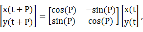
In the second case, we multiply both sides of (R2) by the same quantity to obtain
r(t + P)[cos(P)cos(t) - sin(P)sin(t)] = r(t)[cos(P)cos(t) - sin(P)sin(t)]and analogously for y(t + P), so the conditions (R1) are met.r(t + P)cos(t + P) = cos(P)r(t)cos(t) - sin(P)r(t)sin(t)
x(t + P) = cos(P)x(t) - sin(P)y(t),
Proof. Without loss of generality, let the ellipse be aligned on the coordinate
axes with its center at the origin. Let its dimensions be a and b, with
Q = (a cos(t),b sin(t))for some t that is not a multiple of π. By the distance premise,
a2 = a2cos2(t) + b2sin2(t)Since t is not a multiple of π, we can divide both sides by sin2(t) to geta2[1 - cos2(t)] = b2sin2(t)
is tangent to the line
(8)
if and only if
y = mx + h (9)
Proof. Substituting (9) in (8), we have the quadratic in x
m2a2 + b2 = (mc + h - d)2 (10)
Since the tangency is a single intersection point between the line and the ellipse, this quadratic has a single solution and so its discriminant is zero: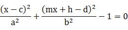
which reduces to (10).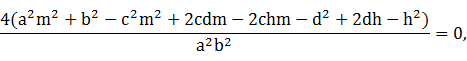
d = h/2 - w2/(8h) and R = h - d, if triangle is acute (w/h < 2)Proof. The equation of a circle of radius R centered on the y-axis at (0,d) isd = 0 and R = w/2, if triangle is obtuse (w/h ≥ 2)
If the isosceles triangle is obtuse or right
x2 + (y - d)2 = R2 (11)
Now assume that the triangle is acute
R = h - dSubstituting the points (±w/2,0) in (11), the results follow.
Analogously, if (h,0) and (0,±w/2) are the vertices of an x-symmetric isosceles triangle, the dimensions and center abscissa of its minimum-area circumellipse are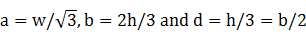
Proof. The equation of an axis-aligned ellipse centered on the y-axis at (0,d) is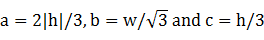
If this ellipse passes through the point (0,h), we have
(12)
Substituting the points (±w/2,0) in (12), we have
b2 = (h - d)2 (13)
The ellipse area πab is minimized when
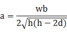
(14)
To prove the case for an x-symmetric isosceles triangle, exchange abscissa and ordinate, y and x, a and b, d and c in the results above.
and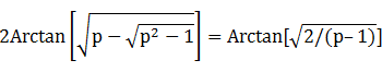
Equivalently,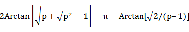
where Atan2 is the two-argument arctangent.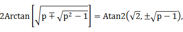
Proof: The tangent half-angle formula is
Substituting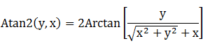
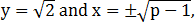 the arctan argument is
after rationalizing the denominator and squaring.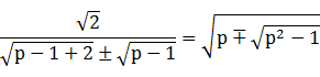
and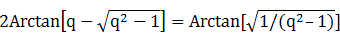
Equivalently,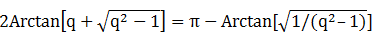
where Atan2 is the two-argument arctangent.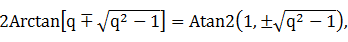
Proof: Let
and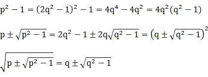
The results follow from Lemma X.
A circumconic of S contains the convex hull of S.Proof. A point in the convex hull of S is either within S, and therefore contained in the circumconic of S, or on a line segment connecting two points of S. Since the circumconic is a circle or ellipse, it is convex and so if it contains the endpoints of a line segment, it also contains all points on that line segment.
[2] Stewart, James,
Single
Variable Calculus, 6th ed., Belmont, CA: Thomson Brooks/Cole, 2008,
p. 579, referenced (along with some funny math jokes) in
[3] Jameson, G.J.O., "Inequalities for the perimeter of an ellipse", Mathematical Gazette, 98 (542): 227-234 (2014), cited in Wikipedia Ellipse article.
[4] Purcell, Edwin J., Calculus, New York: Appleton-Century-Crofts, 1965.
[5] Stewart, op. cit., p. 668.
[6] Stewart, op. cit., p. 686-688.
[7] Michon, Gerard P., "Perimeter of an Ellipse", 2002.
[8] Stewart, op. cit., p. 581.
[9] TimeCoder, "Finding the centroid of a polar curve" Answer #1, 2017.
[10] Bankoff, Leon, "A Mere Coincidence", Mathematics Newsletter, Los Angeles City College, November 1954.
Umehara, M. & Yamada, K., Differential Geometry of Curves and Surfaces, Singapore: World Scientific Publishing, 2017.
Copyright © 2021 Balmoral Software (http://www.balmoralsoftware.com). All rights reserved.